Color figures in the book appear as grayscale images in the print version. Below we provide the color versions of these figures.
Chapter 4
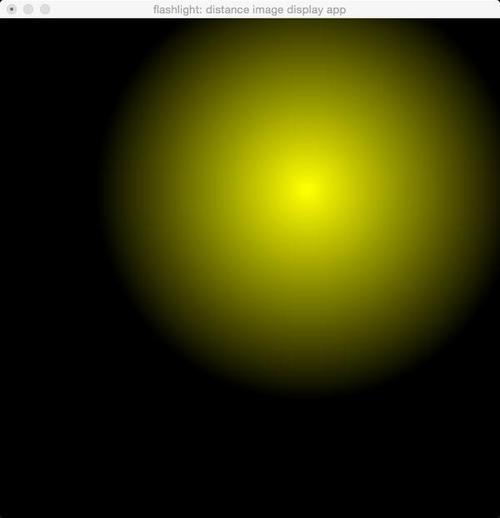
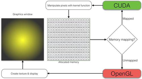
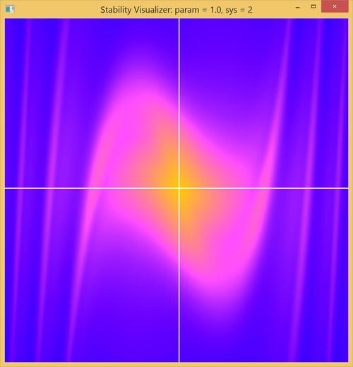
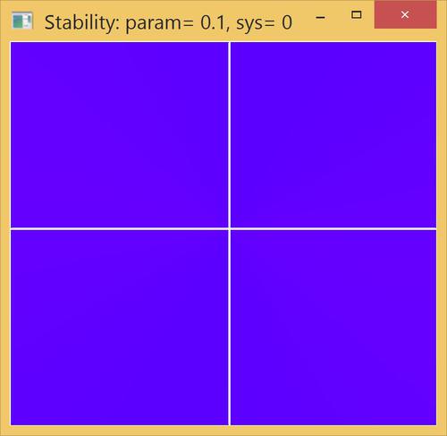
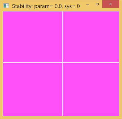
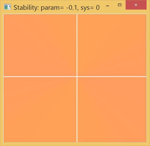
Figure 4.1 Interactive spot of light in the finished applicationFigure 4.2 Illustration of alternating access to device memory that is mapped to CUDA to store computational results and unmapped (i.e., returned to OpenGL control) for display of those resultsFigure 4.3 Stability map with shading adjusted to show a bright central repelling region and surrounding darker attracting regionFigure 4.4 Stability visualization for the linear oscillator with different damping parameter values. (a) For param = 0.1,the dark field indicates solutions attracted to a stable equilibrium. (b) For param = 0.0,the moderately bright field indicates neutral stability. (c) For param = -0.1,the bright field indicates solutions repelled from an unstable equilibrium.
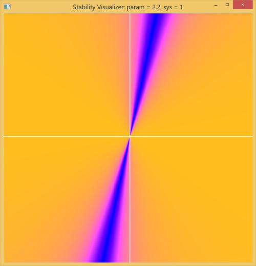
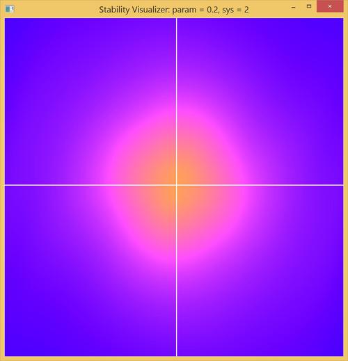
Figure 4.5 Phase plane of a linear oscillator with negative stiffness. A dark sector appears, but the bright field indicates growth away from an unstable equilibrium.Figure 4.6 Phase plane of the van der Pol oscillator. The bright central region indicates an unstable equilibrium. The dark outer region indicates solutions decaying inwards. These results are consistent with the existence of a stable periodic "limit cycle" trajectory in the moderately bright region.
Chapter 5
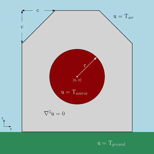
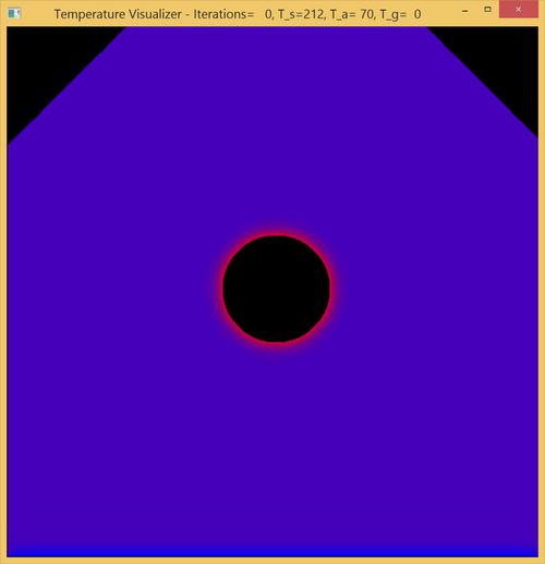
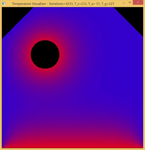
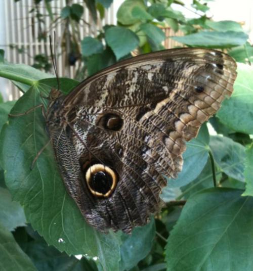
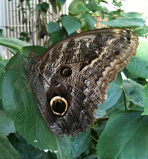
Figure 5.1 Pictorial summary of the equation and boundary conditions to be solved by the heat_2d appFigure 5.2 Initial configuration of the heat_2d appFigure 5.3 The heat_2d app with an edited configurationFigure 5.4 Images of a giant owl butterfly: (a) original and (b) sharpened
Chapter 6
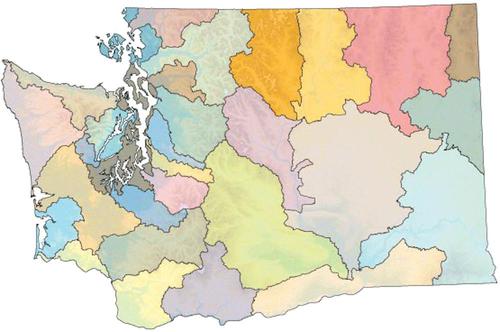
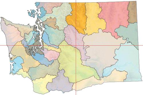
Figure 6.3 Input image showing watershed regions of Washington State. (Map courtesy of United States Geological Survey.)Figure 6.4 Output image with axes locating the centroid
Chapter 7
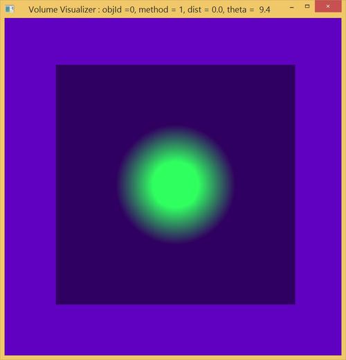
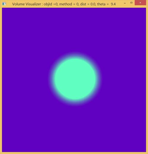
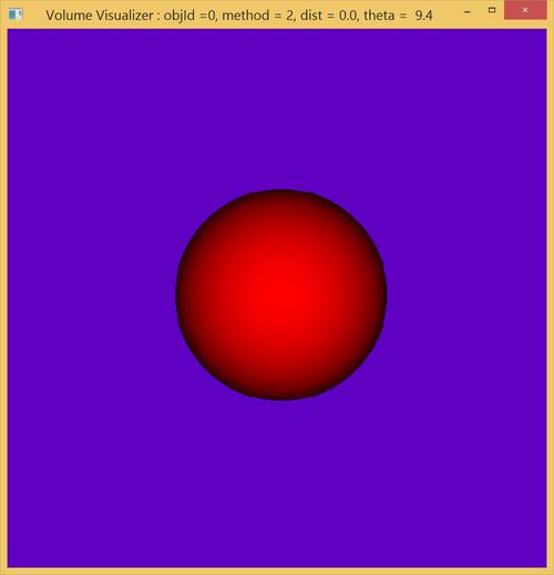
Figure 7.1 Sample images of a 3D distance field (inside a bounding box) produced using the visualization methods provided by vis_3d: (a) slicing, (b) volume rendering, and (c) raycasting
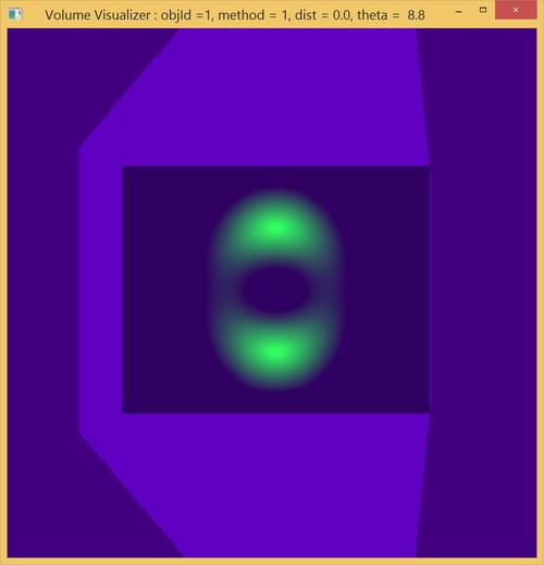
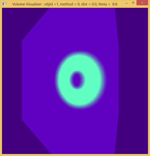
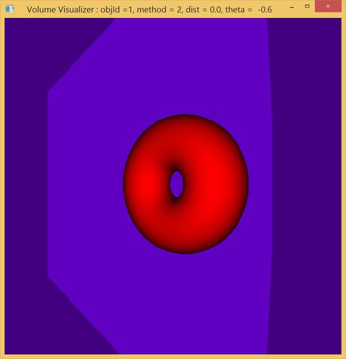
Figure 7.3 Screenshot of vis_3d slice visualization of the 3D distance stack for a torusFigure 7.4 Screenshot of vis_3d volume rendering visualization of the 3D distance stack for a torusFigure 7.5 Screenshot of vis_3d raycast visualization of the 3D distance stack for a torus
Chapter 8
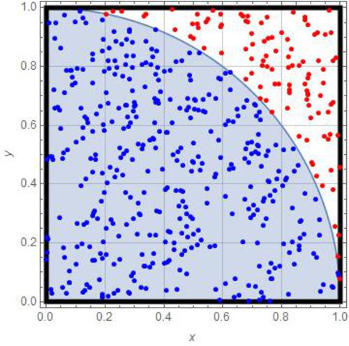
Figure 8.2 For large numbers of points randomly distributed on the unit square, the fraction of the random points that lie within the first quadrant of the unit circle approaches the area ratio π/4 .
Figure 8.4 Rendering of the tricolor trefoil (a) original RGB, (b) sharpened,
(c) colors swapped from RGB to BGR, (d) pixel-wise sum of original and color-swapped images. (Adapted from original image by Jim.belk on Wikimedia Commons, http://commons.wikimedia.org/wiki/File:Tricoloring.png)
Appendix A
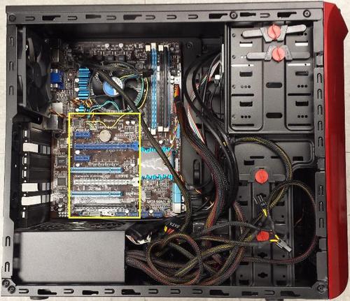
Figure A.3 (a) Desktop PC with case opened to show the hardware.The box indicates the region of peripheral connectors on motherboard.
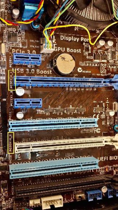
Figure A.3 (b) Blow-up of peripheral connectors including two PCI Express x16 slots. Boxes highlight identifying labels: PCIEX16_1 and PCIEX16_2.
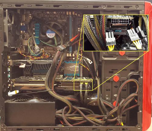
Figure A.4 Desktop computer with a GPU installed in each of the two PCI Express x16 slots: a GeForce GT 610 in the PCIEX16_1 slot and a GeForce GTX 980 in the PCIEX16_2 slot. The smaller rectangle shows the additional power connections to the GTX 980. The larger rectangle shows an enlargement with the power disconnected to make the connectors visible.


